NVIDIA Warp and MjWarp allow MuJoCo simulations to scale to 2,048 parallel GPU environments
MuJoCo Warp (MJWarp) moves compatible MuJoCo models into a GPU-scale regime. This article demonstrates transferring an SO-101 follower arm from a standard MuJoCo workflow to as many as 2,048 parallel MJWarp environments. We examine the technology and validation steps required for this transition.
Figure 1 illustrates the connection between Python and GPU simulation. MuJoCo loads and compiles the MJCF model; MJWarp implements the physics in NVIDIA Warp, which compiles CUDA kernels to advance simulation states on NVIDIA GPUs.
This is the second article in our State of Simulation for Physical AI series. The first article mapped the robot-simulation landscape. Here, we prepare and scale the simulation environment; we do not train a policy. Later installments covering Newton and Isaac Lab address the next integration layers.
Putting it together
The stack operates in layers. NVIDIA Warp serves as the Python kernel language, supporting single instruction, multiple threads (SIMT), autodiff, and PyTorch/JAX interop. MJWarp runs MuJoCo physics on Warp, using the same MJCF format to achieve batched GPU throughput. Your scene, such as the SO-101, provides familiar Menagerie or Robot Studio assets alongside task geometry. The next layer, covering Newton or Isaac Lab, adds a multi-solver API, USD, sensors, managers, and training loops.
Decision shortcut:
- If you need single-robot MPC or teleop, reach for MuJoCo CPU.
- If you need maximum throughput on raw MuJoCo physics, reach for MJWarp or mjlab.
- If you need JAX training recipes, use MuJoCo Playground or MJX with impl=’warp’.
- If you need multi-solver plus Isaac Lab integration, wait for the Newton post in this series.
Start with one useful Warp Kernel
NVIDIA Warp is a Python framework for writing high-performance, GPU-accelerated kernels. Developers author statically typed kernels in Python and compile them for CPU or CUDA execution. The first launch builds and caches a native module; later launches reuse it. The kernel language is a performance-oriented subset of Python, while ordinary Python remains responsible for configuration, allocation, and launch orchestration.
This small robotics-oriented kernel advances point positions under gravity. One logical thread handles one point, so the same code scales from two points to millions without introducing GPU terminology into the control flow.
The three value propositions of Warp are:
- Performance: Native-CUDA speed via JIT compilation, kernel fusion, and CUDA Graphs.
- Ease of use: Pure Python authoring with built-in vectors, matrices, quaternions, BVHs, hash grids, sparse matrices, and tile primitives.
- Capability: Differentiable kernels and DLPack-style interop so simulation can sit inside an ML training loop.
import numpy as np
import warp as wp

@wp.kernel
def integrate(
   positions: wp.array[wp.vec3],
   velocities: wp.array[wp.vec3],
   dt: float,
):
   i = wp.tid()
   velocities[i] += wp.vec3(0.0, 0.0, -9.81) * dt
   positions[i] += velocities[i] * dt

wp.init()
device = "cuda:0" if wp.is_cuda_available() else "cpu"
start = np.array([[0.0, 0.0, 0.5], [0.2, 0.0, 0.5]], dtype=np.float32)
positions = wp.array(start, dtype=wp.vec3, device=device)
velocities = wp.zeros_like(positions)

wp.launch(
   integrate,
   dim=len(start),
   inputs=[positions, velocities, 0.01],
   device=device,
)
wp.synchronize_device(device)
print(positions.numpy())
Three properties make this useful in robotics
- Explicit parallel work. wp.tid() identifies the point, contact, body, or world owned by the current logical thread.
- Explicit device arrays. An array lives on the selected device. Calling .numpy() on a CUDA array synchronizes and copies it to CPU memory; it is not a zero-copy path. For a device-resident PyTorch or JAX pipeline, use Warp’s framework adapters or DLPack-compatible sharing instead.
- Composable kernel launches. A program can launch a sequence of focused kernels and capture supported CUDA work into a graph to reduce repeated dispatch overhead. Graph capture replays launches against existing buffers; it does not fuse arbitrary kernels.
Differentiability and Determinism
Two further Warp capabilities are worth knowing, even though neither is used in the SO-101 workflow in this article. Warp kernels are differentiable: a wp.Tape records the forward kernel launches made inside its context and replays their adjoints in reverse when backward() is called. This is why teams build differentiable geometry, CFD, and custom physics in Warp, including CAE workflows for simulation and design optimization. Warp also supports deterministic execution, introduced in Warp 1.15: GPU atomics are scheduler-dependent by default, so repeated launches of the same kernel can differ slightly, and the opt-in deterministic modes trade some performance for reproducible ordering in simulation, validation, and regression tests. These are Warp capabilities, not guarantees of differentiability or determinism for an entire MJWarp rollout. See the Warp documentation on differentiability and deterministic execution for the details.
Try Warp: pip install warp-lang (≥ 1.15 for GPU determinism), then python -m warp.examples.browse, or the tutorial notebooks.
What is MuJoCo Warp (MJWarp)?
A robot simulator repeatedly computes what happens next: given the current joint positions, velocities, controls, and contacts, it advances the scene by one small timestep. In this article, a world means one independent copy of that scene and its state. One world might contain the SO-101 arm reaching for a cube; another can contain the same arm starting from a slightly different pose.
MuJoCo and MJWarp can run the same compatible robot and task, but they organize the work differently. MuJoCo naturally suits developing and inspecting one or a few CPU worlds. MJWarp is a NVIDIA Warp implementation of MuJoCo’s physics pipeline that places the model and a batch of independent states on NVIDIA GPUs; one call to mjw.step advances the entire batch.
MJWarp’s value is not necessarily a faster step for one world. It is the ability to advance hundreds or thousands together, giving the GPU enough parallel work to improve aggregate throughput, the total world-steps completed per second. That favors reinforcement learning and large-scale sampling, where collecting experience matters more than minimizing one environment’s latency.
This blog covers the following:
- validate one MuJoCo world
- move it to MJWarp, form a batch
- verify it, and measure it correctly
Solver tuning, Jacobian representation, and specialized multi-GPU or determinism topics are not required for this migration and can be covered separately.
Then, the distinction is precise:
- Latency is wall-clock time for one simulation step.
- Aggregate throughput is the total number of world-steps completed per measured wall-clock second.
Basic usage: structs, batch sizes, and a minimal step
The core API transition is small:
- mujoco.MjModel becomes mjw.put_model(mjm) to create a device model.
- mujoco.MjData becomes mjw.put_data(mjm, mjd, …) to preserve and batch an existing state.
- mujoco.mj_step(mjm, mjd) becomes mjw.step(m, d) to advance every world in d.
- Host arrays such as mjd.ctrl become batched device arrays such as d.ctrl with shape (nworld, nu).
Use mjw.make_data() when default or fresh state is intended. Use mjw.put_data() when the exact initialized MuJoCo state must cross the migration boundary.
Allocating batched resources requires defining the following parameters:
- nworld: Total number of parallel environments.
- nconmax: Expected contacts per individual world (overall capacity ≈ nconmax * nworld).
- naconmax: Alternative setting: global maximum contacts across all environments combined (takes precedence if both are defined).
- njmax: Hard upper limit on constraints per world.
Performance tuning
1. CUDA graph capture: mjw.step is many kernel launches; capture once, replay often:
with wp.ScopedCapture() as capture:
     mjw.step(m, d)
wp.capture_launch(capture.graph)
2. Size nconmax / naconmax / njmax tightly: memory and work scale with them. Tune with mjwarp-testspeed: –measure_alloc and watch overflows in mjwarp-viewer.
Additional tuning considerations. After sizing contact and constraint buffers, test solver iteration limits without changing task behavior. Meshes and CCD settings can increase memory use; nccdmax / naccdmax can reduce CCD buffer allocation when the measured contact counts allow it. MJWarp’s compact solver uses MuJoCo’s Newton constraint solver and sleeping, not the separate Newton physics-engine framework. Compact-solver and multi-GPU configuration are beyond this walkthrough; consult the MJWarp performance-tuning documentation.
To train policies on MJWarp physics:
- Isaac Lab via Newton
- mjlab (manager API directly on MJWarp + PyTorch)
- MuJoCo Playground via MJX (impl=’warp’)
Install / try: pip install mujoco-warp · mjwarp-viewer path/to/scene.xml · Colab tutorial
Workflow to migrate a MuJoCo scene to MjWarp
The scene. Nothing here is MJWarp-specific yet: an SO-101 arm, a table, and two cubes to stack, written as ordinary MJCF.
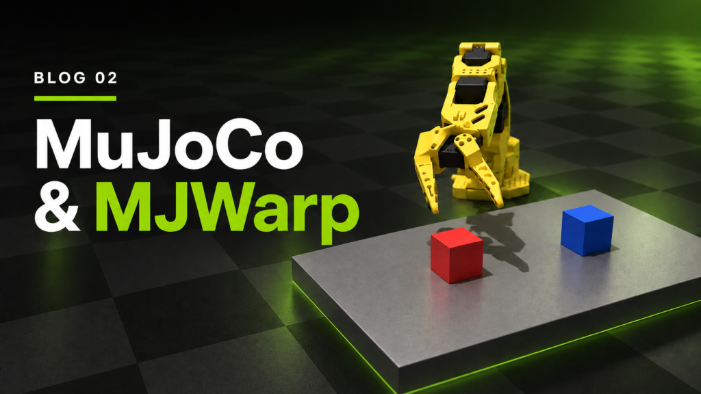
Figure 2 shows the SO-101 pick-and-place scene, rendered from the MuJoCo CPU simulation. The task is to grasp the red 44 mm cube and stack it on the blue cube; the same robot and scene are used for MJWarp validation.
<mujoco model="Source Read original →