For the mathematician and data scientist, the landscape of research is shifting from static archives to dynamic, queryable knowledge bases. Recent work demonstrates how to transform the amphora/ResearchMath-14k dataset into a functional semantic search engine and a status classifier. By leveraging open-source tools, creators can now build systems that not only retrieve relevant papers based on meaning rather than keywords but also predict whether a problem remains unsolved. This approach turns a raw collection of arXiv entries into an intelligent assistant for navigating complex mathematical taxonomy.
Setting the stage
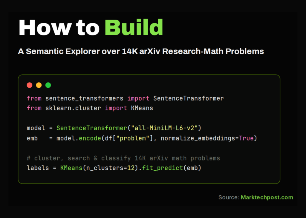
The foundation of this project is the amphora/ResearchMath-14k dataset, a curated collection of research-level mathematics problems sourced from arXiv. The initial phase involves loading this data and establishing a clean computational environment. Key configuration parameters include a sample size of 4,000 records, a random seed of 42 for reproducibility, and the sentence-transformers/all-MiniLM-L6-v2 model for generating embeddings.
!pip -q install -U datasets sentence-transformers scikit-learn umap-learn \
   pandas matplotlib seaborn wordcloud 2>/dev/null
import warnings, numpy as np, pandas as pd
warnings.filterwarnings("ignore")
import matplotlib.pyplot as plt
import seaborn as sns
sns.set_theme(style="whitegrid", palette="deep")
SAMPLE_SIZE = 4000
RANDOM_STATE = 42
EMB_MODEL   = "sentence-transformers/all-MiniLM-L6-v2"
The code imports essential libraries for data manipulation, visualisation, and machine learning. It suppresses warnings and configures the plotting library with a clean aesthetic before proceeding to load the dataset from Hugging Face.
Inspecting the corpus
Loading the dataset converts it into a pandas DataFrame for easier analysis. The initial inspection reveals the number of rows and available columns. A crucial filtering step removes problem statements shorter than 20 characters, ensuring that subsequent analysis operates on substantive text rather than noise.
from datasets import load_dataset
ds = load_dataset("amphora/ResearchMath-14k", split="test")
df = ds.to_pandas()
print("Rows:", len(df))
print("Columns:", list(df.columns))
df.head(3)
TEXT_COL = "self_contained_problem"
df = df[df[TEXT_COL].astype(str).str.len() > 20].reset_index(drop=True)
Visualising distribution and structure
Understanding the data requires visualising how problems are distributed across open-status labels and mathematical fields. Charts display the frequency of problem statuses, the top-level math fields, and the length distribution of the problem statements. A heatmap is generated to reveal correlations, showing how the proportion of open versus solved problems varies across different areas of mathematics.
print("\n--- open_status distribution ---")
print(df["open_status"].value_counts(dropna=False))
print("\n--- taxonomy_level_1 (math fields) ---")
print(df["taxonomy_level_1"].value_counts())
fig, axes = plt.subplots(1, 3, figsize=(20, 6))
df["open_status"].value_counts().plot(
   kind="bar", ax=axes[0], color="steelblue")
axes[0].set_title("Problem status"); axes[0].tick_params(axis="x", rotation=30)
df["taxonomy_level_1"].value_counts().plot(
   kind="barh", ax=axes[1], color="seagreen")
axes[1].set_title("Top-level math field"); axes[1].invert_yaxis()
df["doc_len"] = df[TEXT_COL].str.split().apply(len)
axes[2].hist(df["doc_len"].clip(upper=400), bins=40, color="indianred")
axes[2].set_title("Problem length (words, clipped @400)")
plt.tight_layout(); plt.show()
ct = pd.crosstab(df["taxonomy_level_1"], df["open_status"], normalize="index")
plt.figure(figsize=(10, 6))
sns.heatmap(ct, annot=True, fmt=".2f", cmap="rocket_r")
plt.title("Fraction of each status within each field")
plt.tight_layout(); plt.show()
Extracting field-specific terminology
To understand the unique vocabulary dominating specific branches of mathematics, the code applies TF-IDF (Term Frequency-Inverse Document Frequency). This technique calculates the importance of terms within each top-level field. The output lists the most significant keywords or phrases for each category, providing a linguistic fingerprint of the research landscape.
from sklearn.feature_extraction.text import TfidfVectorizer
def top_terms_per_group(frame, group_col, text_col, k=8):
   out = {}
   for g, sub in frame.groupby(group_col):
       if len(sub) < 20:
           continue
       vec = TfidfVectorizer(max_features=3000, stop_words="english",
                             ngram_range=(1, 2), min_df=3)
       X = vec.fit_transform(sub[text_col])
       scores = np.asarray(X.mean(axis=0)).ravel()
       terms = np.array(vec.get_feature_names_out())
       out[g] = terms[scores.argsort()[::-1][:k]].tolist()
   return out
for field, terms in top_terms_per_group(df, "taxonomy_level_1", TEXT_COL).items():
   print(f"\n{field:35s} -> {', '.join(terms)}")
Building the semantic search engine
The core of the project is transforming text into semantic embeddings using the SentenceTransformer model. These high-dimensional vectors capture the meaning of mathematical problems. The system reduces these vectors to two dimensions using UMAP (Uniform Manifold Approximation and Projection) to visualise the problem landscape. A K-Means clustering algorithm is then applied to group similar problems, with performance against human labels measured using ARI and NMI scores.
from sentence_transformers import util
def search(query, k=5):
q = model.encode([query], normalize_embeddings=True)
sims = util.cos_sim(q, emb)[0].cpu().numpy()
idx = sims.argsort()[::-1][:k]
print(f'\n=== Query: "{query}" ===')
for rank, i in enumerate(idx, 1):
row = work.iloc[i]
print(f"\n[{rank}] sim={sims[i]:.3f} | {row['taxonomy_level_1']} "
f"| status={row['open_status']}")
print(" ", row[TEXT_COL][:260].replace("\n", " "), "...")
search("rational points on hyperelliptic curves")
search("multiplicativity of maximal output p-norm of a quantum channel")
from sklearn.linear_model import LogisticRegression
from sklearn.model_selection import train_test_split
from sklearn.metrics import classification_report, ConfusionMatrixDisplay
y = work["Source Read original →Stay ahead of AI. Get the most important stories delivered to your inbox — no spam, no noise.
More in AI Guides & Tutorials