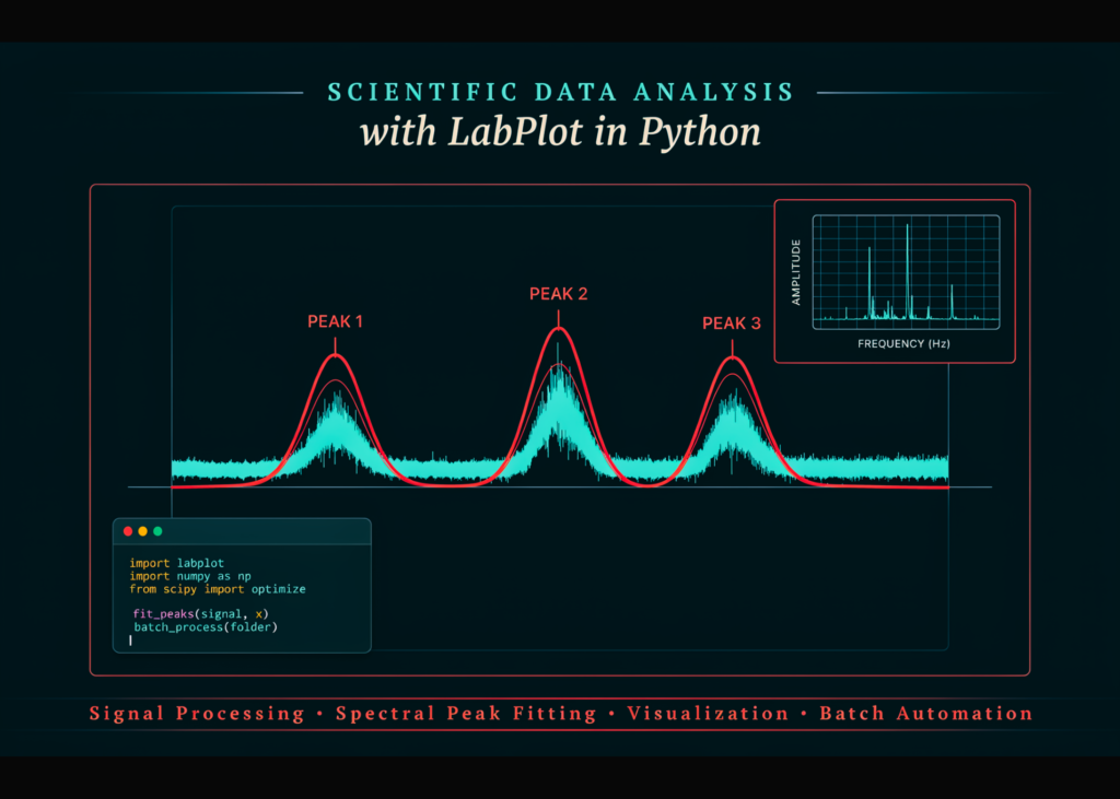
The tutorial demonstrates how to build a Python workflow that mirrors the LabPlot software architecture, covering signal processing, spectral peak fitting, and batch automation.
Core architecture
The code preserves the structure of LabPlot’s aspect tree, analysis kernels, and project model. It creates reusable components to import tabular data, compute descriptive statistics, smooth and differentiate signals, perform Fourier analysis, detect peaks, integrate curves, reduce data, and fit nonlinear models with statistical diagnostics.
The workflow applies these tools to a realistic spectroscopy example. The process removes periodic interference, identifies overlapping peaks, fits a multi-Gaussian model, inspects residuals, and visualizes results through themed worksheets. Figures export correctly, and project data saves in LabPlot-compatible .lml-style files.
The final step extends the workflow to batch processing. This allows analysis of multiple temperature-dependent spectra and fitting of secondary trends across resulting measurements.
Implementation details
The setup configures the Python environment, establishes reproducibility, and creates an output directory. It recreates LabPlot’s core aspect-tree using projects, spreadsheets, columns, plot designations, and column modes. An AsciiFilter workflow imports structured text data into the LabPlot-style data model.
Analysis functions include Savitzky-Golay smoothing, differentiation for noisy data, and integration using rectangle, trapezoid, or Simpson’s methods. A Fourier Transform module calculates amplitude, magnitude, power, or decibels using five window types.
Code structure
The initial script imports necessary libraries including numpy, pandas, matplotlib, and scipy. It sets a random seed for reproducibility and checks for the Google Colab environment. The code defines an output path, creating the directory if it does not exist.
It attempts to import a custom SDK named pylabplot. If the import fails, the system defaults to an emulation mode. A banner function prints environment details, listing numpy, scipy, and matplotlib versions alongside the Colab status.
Classes define the data model. PlotDesignation acts as an enum for X, Y, and Z axes, including error variants. ColumnMode handles data types like Double, Text, Integer, BigInt, and DateTime. The AbstractAspect class manages the tree structure with name, comment, and parent references.
The Column class serves as the fundamental data source. It stores a typed vector and a plot designation. The statistics method calculates twenty quantities found in LabPlot’s Column Statistics dialog, including count, minimum, maximum, arithmetic and geometric means, variance, skewness, and entropy.
A sparkline method generates a text-based visual representation of the data within the column header. The Spreadsheet class manages multiple columns, allowing retrieval by index or name. It can append columns and convert the entire sheet to a pandas DataFrame.
The Project class initializes the root element with a name and author, defaulting to version 2.12.1. The AsciiFilter class handles text import with auto-detection of separators, support for comment characters, and limits for rows and columns.
The readDataFromFile method opens a file, strips newlines, and filters out comment lines. It splits lines based on the detected separator. The code maps values to float, handling errors by appending NaN. It then creates Column objects for the data, assigning X or Y designations based on the column index.
Subsequent classes handle specific analysis tasks. The nsl_smooth class uses Savitzky-Golay filtering. The nsl_diff class computes derivatives, optionally smoothing the data first to reduce noise. The simpson function performs composite integration on non-uniform grids using Cartwright’s formula.
The nsl_int class integrates data using rectangle, trapezoid, or Simpson’s methods. It can calculate cumulative sums and absolute values. The nsl_dft class begins the Fourier Transform implementation, defining window functions such as rectangular, hann, and hamming.
What it means
Researchers can now replicate the specific data handling and visualization logic of LabPlot within a standard Python environment. This allows for custom batch processing of spectroscopy data without relying on the proprietary software interface.