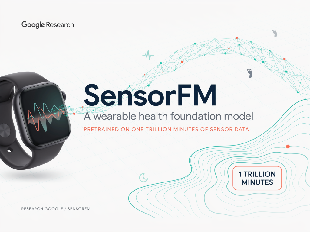
Google Research has released SensorFM, a foundation model for wearable health data trained on 1 trillion minutes of sensor readings from 5 million people.
Current wearable health models typically target a single outcome, such as sleep tracking or heart rate variance. This approach breaks down when trying to cover 35 different health endpoints simultaneously. Labeling that much data is expensive, and retrospective annotation is often impossible.
What is SensorFM?
The new system is a Large Sensor foundation Model designed for wearable time-series representation learning. It ingests 34 one-minute aggregate features drawn from five sensors: PPG, accelerometer, EDA, skin temperature, and altimeter. These features are organised into seven categories over a 24-hour context window.
The backbone is a ViT-1D encoder trained with a masked-autoencoder objective and a patch size of [20, 1]. Pretraining used 5,000,000 consented participants, sampled between September 2024 and September 2025. That corpus spans 100+ countries, all 50 U.S. states, and 20+ Fitbit and Pixel Watch models. It totals over two billion hours, or more than one trillion minutes.
Four variants exist, each paired with a proportional data volume.
| Variant | Parameters | Encoder hidden / layers | Proportional data | Sensor-hours |
|---|---|---|---|---|
| XXS | 138,740 | 64 / 2 | 5K subjects | 2×10⁶ |
| XS | 933,204 | 128 / 4 | 50K subjects | 2×10⁷ |
| S | 7,290,068 | 256 / 8 | 500K subjects | 2×10⁸ |
| B | 110,763,412 | 768 / 12 | 5M subjects | 2×10⁹ |
Evaluation uses separate data. It covers 13,985 subjects across three prospective IRB-approved studies. Those are metabolic, cardiac and respiratory health (N = 1,655), sleep (N = 6,377), and mental health (N = 5,953). The 35 tasks cover cardiovascular (6), metabolic (8), mental health (8), sleep (3), demographics (4), and lifestyle (6).
The Scaling Case
With that setup, the first question is whether scale buys anything measurable. The research team swept four model sizes against four data volumes.
SensorFM-B on the 5M corpus cuts reconstruction validation loss by 31% versus SensorFM-XXS. Generative loss drops 28% on average. Downstream, it gains ΔAUC = 0.09 on classification and Δr = 0.21 on regression. Across variants, B wins 33 of 35 tasks, and XXS ranks last on 33 of 35.
The failure case is equally informative. SensorFM-B trained on only 5K subjects posts a 1.082 validation loss. That is worse than every smaller variant at the same volume. Pretraining was stopped early because the model overfit.
Consequently, all headline results assume data volumes scaled proportionally to capacity. Along that co-scaled diagonal, mean ROC AUC moves .664, .681, .710, .752. Mean Pearson r moves .386, .435, .536, .612. The above figure shows the trend has not saturated.
AIM: Handling Missing Data as Signal
Scaling alone does not explain those numbers. Real streams fragment during charging, off-wrist periods, and power-saving modes. Conventional methods either impute the gaps, injecting bias, or drop the windows, discarding data.
SensorFM instead uses Adaptive and Inherited Masking (AIM), introduced by Xu et al. in LSM-2. The applied mask is the union of the inherited missingness mask and the artificial mask. Loss is computed only on artificially masked patches that had ground truth. Two-stage token masking, using token dropout and attention masking, keeps this efficient.
Because the decoder learns to reconstruct ablated observations, imputation and forecasting come for free.
| Generative task | Mean fill | NN fill | Linear interp. | SensorFM-B |
|---|---|---|---|---|
| Random imputation, 80% | 0.915 | 1.020 | 0.854 | 0.215 |
| Temporal interpolation, 60 min | 0.904 | 0.943 | 0.777 | 0.468 |
| Temporal extrapolation, 60 min | 0.937 | 1.102 | 1.102 | 0.563 |
| Signal imputation, 12/26 channels | 1.025 | 1.025 | 1.025 | 0.170 |
Reconstruction MSE on the held-out test set, lower is better.
Against the best baseline, SensorFM improves random imputation by 74.8%. Sensor signal imputation improves by 83.7%.
Hands-On: Adapting the Embeddings
Turning that representation into predictions is straightforward. The encoder stays frozen. Embeddings are aggregated per person, using the mean and standard deviation across days. Those reduce to 50 principal components. A linear head then trains under five-fold, person-independent cross-validation.
import numpy as np
from sklearn.decomposition import PCA
from sklearn.linear_model import LogisticRegression
from sklearn.model_selection import StratifiedKFold
from sklearn.metrics import roc_auc_score

def person_level(emb, pid):
    """Collapse day-level embeddings into one vector per participant."""
    people = np.unique(pid)
    feats = []
    for p in people:
        e = emb[pid == p]                    # (n_days, d)
        feats.append(np.concatenate([e.mean(axis=0), e.std(axis=0)]))
    return np.nan_to_num(np.stack(feats)), people   # pandas std() is NaN at 1 day

X, people = person_level(emb, pid)           # emb: frozen SensorFM embeddings
y = labels[people]                           # one label per participant

aucs = []
for tr, te in StratifiedKFold(5, shuffle=True, random_state=0).split(X, y):
    pca = PCA(n_components=50).fit(X[tr])    # PCA-50, fit on the train fold only
    clf = LogisticRegression(max_iter=400)   # paper: AdamW, lr 5e-3, wd 1e-4, 400 steps
    clf.fit(pca.transform(X[tr]), y[tr])
    p = clf.predict_proba(pca.transform(X[te]))[:, 1]
    aucs.append(roc_auc_score(y[te], p))
print(np.mean(aucs))
This linear probe beats a supervised feature-engineered baseline on 34 of 35 tasks. Selected results follow.
| Task | Metric | Demos. only | Feat. Eng. | SensorFM-B |
|---|---|---|---|---|
| Age | r | – | .662 | .920 |
| Mental Health Med. | ROC | .594 | .773 | .819 |
| PHQ-8 | r | .303 | .354 | .450 |
| Insulin Resistance | ROC | .717 | .710 | .761 |