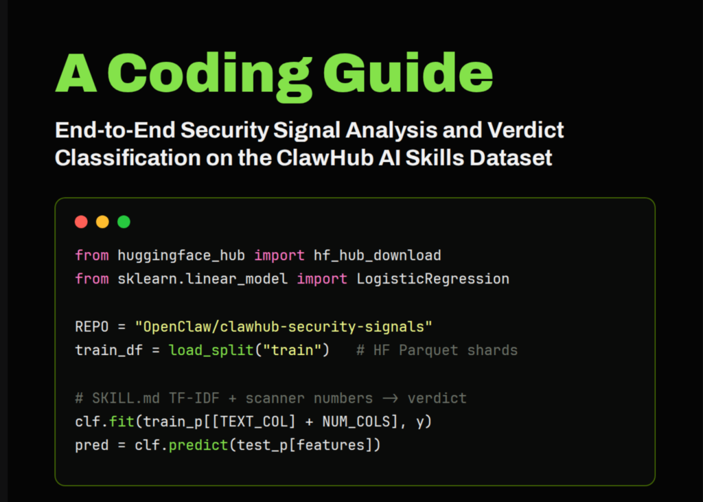
In this tutorial, we use the ClawHub Security Signals dataset to examine how different security scanners assess AI skills and related files. We load the dataset directly from the Hugging Face Parquet conversion to avoid compatibility issues with newer dataset metadata, then inspect the main columns, verdict distribution, scanner outputs, and severity labels. After exploring scanner disagreement and overlap patterns, we build a practical machine learning pipeline that combines SKILL.md text with numerical scanner signals to predict the final ClawScan verdict. It gives us a complete workflow for loading, analyzing, visualizing, and modeling security signal data in a Colab-ready environment.
Setting Up the Colab Environment and Imports for Security Signal Analysis
!pip -q install -U "huggingface_hub>=0.23" pyarrow scikit-learn pandas numpy matplotlib seaborn
import warnings, numpy as np, pandas as pd
warnings.filterwarnings("ignore")
import matplotlib.pyplot as plt
import seaborn as sns
sns.set_theme(style="whitegrid")
from huggingface_hub import HfApi, hf_hub_download
from sklearn.feature_extraction.text import TfidfVectorizer
from sklearn.linear_model import LogisticRegression
from sklearn.compose import ColumnTransformer
from sklearn.pipeline import Pipeline
from sklearn.preprocessing import StandardScaler, FunctionTransformer
from sklearn.impute import SimpleImputer
from sklearn.metrics import (classification_report, confusion_matrix,
                            cohen_kappa_score, jaccard_score)
SAMPLE_SIZE = 20000
RANDOM_STATE = 42
We install all the required libraries and import the main packages needed for data loading, analysis, visualization, and machine learning. We also configure warnings and set the plotting style to keep the notebook output clean and readable. Finally, we define the sample size and random seed to make the experiment controlled and reproducible.
Loading the ClawHub Security Signals Dataset from the Hugging Face Parquet Conversion
REPO = "OpenClaw/clawhub-security-signals"
REV  = "refs/convert/parquet"
print("Listing Parquet files on the Hub...")
api = HfApi()
all_files = api.list_repo_files(REPO, repo_type="dataset", revision=REV)
parquet_files = [f for f in all_files if f.endswith(".parquet")]
def load_split(split):
   """Download + concat all Parquet shards for a given split into a DataFrame."""
   shards = [f for f in parquet_files
             if f.split("/")[-2] == split]
   if not shards:
       raise ValueError(f"No parquet files for split '{split}'. Found: {parquet_files[:5]}")
   frames = []
   for f in shards:
       local = hf_hub_download(REPO, f, repo_type="dataset", revision=REV)
       frames.append(pd.read_parquet(local))
   return pd.concat(frames, ignore_index=True)
print("Downloading train + test splits (first run pulls the data)...")
train_df = load_split("train")
test_df  = load_split("test")
if SAMPLE_SIZE:
   train_df = train_df.sample(min(SAMPLE_SIZE, len(train_df)),
                              random_state=RANDOM_STATE).reset_index(drop=True)
print(f"\nTrain rows in use: {len(train_df):,} | Test rows: {len(test_df):,}")
print("Columns:", list(train_df.columns))
We connect to the Hugging Face dataset repository and list the available Parquet files from the converted dataset branch. We create a helper function to download and combine the Parquet shards for each split into a single pandas DataFrame. We then load the train and test splits, optionally sample the training data, and print the dataset size and column names.
Exploring Verdict Distribution and Scanner Agreement with Jaccard and Cohen’s Kappa
print("\n=== ClawScan verdict distribution (train) ===")
print(train_df["clawscan_verdict"].value_counts(normalize=True).mul(100).round(2))
print("\n=== SkillSpector severity distribution ===")
print(train_df["skillspector_severity"].value_counts(dropna=False))
sample = train_df.iloc[0]
print(f"\nExample skill: {sample['skill_slug']} (v{sample['skill_version']})")
print(f"Verdict: {sample['clawscan_verdict']} | Summary: {sample['clawscan_summary']}")
print("SKILL.md (first 400 chars):\n", str(sample["skill_md_content"])[:400])
POSITIVE = {"suspicious", "malicious"}
def is_pos(series):
   return series.fillna("").isin(POSITIVE).astype(int)
an = train_df.copy()
an["vt_pos"]     = is_pos(an["virustotal_status"])
an["static_pos"] = is_pos(an["static_status"])
an["spec_pos"]   = is_pos(an["skillspector_status"])
print("\n=== Scanner positive rates ===")
for col, name in [("vt_pos","VirusTotal"),("static_pos","Static"),("spec_pos","SkillSpector")]:
   print(f"  {name:12s}: {an[col].mean()*100:5.2f}% positive")
def pattern(r):
   tags = []
   if r.vt_pos: tags.append("VT")
   if r.static_pos: tags.append("Static")
   if r.spec_pos: tags.append("SkillSpector")
   return "None" if not tags else " + ".join(tags)
an["pattern"] = an.apply(pattern, axis=1)
print("\n=== Positive-signal overlap patterns ===")
print(an["pattern"].value_counts(normalize=True).mul(100).round(2))
print("\n=== Pairwise agreement (low = scanners inspect different surfaces) ===")
pairs = [("vt_pos","static_pos","VT vs Static"),
        ("vt_pos","spec_pos","VT vs SkillSpector"),
        ("static_pos","spec_pos","Static vs SkillSpector")]
for a, b, label in pairs:
   j = jaccard_score(an[a], an[b], zero_division=0)
   k = cohen_kappa_score(an[a], an[b])
   print(f"  {label:26s} Jaccard={j:.3f}  Cohen's kappa={k:.3f}")
We perform the main exploratory analysis on the ClawHub Security Signals dataset. We inspect verdict distributions, severity labels, example skill metadata, and the beginning of a SKILL.md file to understand the data structure. We also convert scanner outputs into positive flags and compare VirusTotal, static analysis, and SkillSpector through positive rates, overlap patterns, Jaccard scores, and Cohen’s kappa.
Visualizing Verdict Distribution, Scanner Positive Rates, and Overlap Patterns
fig, axes = plt.subplots(2, 2, figsize=(14, 10))
order = ["clean","suspicious","malicious"]
sns.countplot(data=train_df, x="clawscan_verdict", order=order, ax=axes[0,0], palette="viridis")
axes[0,0].set_title("ClawScan verdict distribution"); axes[0,0].set_yscale("log")
rates = {"VirusTotal":an["vt_pos"].mean(), "Static":an["static_pos"].mean(),
        "SkillSpector":an["spec_pos"].mean()}
axes[0,1].bar(rates.keys(), [v*100 for v in rates.values()], color="#d95f02")
axes[0,1].set_title("Scanner positive rate (%)"); axes[0,1].set_ylabel("% flagged")
pc = an["pattern"].value_counts()
axes[1,0].barh(pc.index, pc.values, color="#7570b3")
axes[1,0].set_title("Positive-signal overlap patterns"); axes[1,0].invert_yaxis()
sns.boxplot(data=train_df, x="clawscan_verdict", y="skillspector_score",
           order=order, ax=axes[1,1], palette="viridis")
axes[1,1].set_title("SkillSpector score by verdict")
plt.tight_layout(); plt.show()
We create visualizations to make the dataset patterns easier to understand. We plot the ClawScan verdict distribution, scanner positive rates, positive-signal overlap patterns, and SkillSpector score differences across verdict categories. These charts help us quickly see class imbalance, scanner behavior, and the relationship between numerical security scores and final verdicts.
Building a Logistic Regression Pipeline on SKILL.md Text and Scanner Signals to Predict ClawScan Verdicts
TEXT_COL = "skill_md_content"
NUM_COLS = ["skillspector_score", "static_finding_count",
           "skillspector_issue_count", "virustotal_malicious_count"]
TARGET   = "clawscan_verdict"
def prep(df):
   out = df.copy()
   out[TEXT_COL] = out[TEXT_COL].fillna("").astype(str).str.slice(0, 6000)
   for c in NUM_COLS:
       out[c] = pd.to_numeric(out[c], errors="coerce")
   return out
train_p, test_p = prep(train_df), prep(test_df)
get_text = FunctionTransformer(lambda X: X[TEXT_COL].values, validate=False)
text_pipe = Pipeline([
   ("select", get_text),
   ("tfidf", TfidfVectorizer(max_features=20000, ngram_range=(1,2),
                             min_df=3, sublinear_tf=True)),
])
num_pipe = Pipeline([
   ("impute", SimpleImputer(strategy="constant", fill_value=0)),
   ("scale", StandardScaler()),
])
features = ColumnTransformer([
   ("text", text_pipe, [TEXT_COL]),
   ("num", num_pipe, NUM_COLS),
])
clf = Pipeline([
   ("features", features),
   ("model", LogisticRegression(max_iter=2000, C=4.0,
                                class_weight="balanced",
                                multi_class="multinomial")),
])
print("\nTraining classifier (SKILL.md text + scanner numbers -> verdict)...")
clf.fit(train_p[[TEXT_COL] + NUM_COLS], train_p[TARGET])
pred = clf.predict(test_p[[TEXT_COL] + NUM_COLS])
print("\n=== Test-set classification report ===")
print(classification_report(test_p[TARGET], pred, digits=3))
cm = confusion_matrix(test_p[TARGET], pred, labels=order)
plt.figure(figsize=(6,5))
sns.heatmap(cm, annot=True, fmt="d", cmap="Blues", xticklabels=order, yticklabels=order)
plt.title("Confusion matrix (test split)"); plt.xlabel("Predicted"); plt.ylabel("Actual"); plt.show()
test_out = test_p[["skill_slug", TARGET, "clawscan_summary"]].copy()
test_out["pred"] = pred
errors = test_out[test_out[TARGET] != test_out["pred"]].head(8)
print("\n=== Sample misclassifications ===")
for _, r in errors.iterrows():
   print(f"- {r['skill_slug']:35s} true={r[TARGET]:10s} pred={r['pred']:10s}")
print("\nDone. Set SAMPLE_SIZE=None for the full dataset.")
We prepare the text and numerical features for training a machine learning classifier. We build a pipeline that uses TF-IDF features from SKILL.md content, along with scanner-related numeric fields, and then trains a balanced logistic regression model to predict the ClawScan verdict. We evaluate the model using a classification report, a confusion matrix, and sample misclassifications to understand where the classifier performs well and where it fails.
Conclusion
In conclusion, we completed an end-to-end analysis of the ClawHub Security Signals dataset, from robust data loading to test-set evaluation of a verdict classifier. We examined how VirusTotal, static analysis, and SkillSpector signals differ, visualized their patterns, and used both textual and numerical features to train a balanced logistic regression model. This workflow helps us understand how security verdicts are distributed, and also how multiple scanner signals can be combined into a simple predictive system. We can extend this further by using the full dataset, trying stronger text models, or adding deeper feature engineering around scanner summaries and skill metadata.
Check out the Full Codes with Notebook. Also, feel free to follow us on Twitter and don’t forget to join our 150k+ ML SubReddit and Subscribe to our Newsletter. Wait! are you on telegram? now you can join us on telegram as well.
Need to partner with us for promoting your GitHub Repo OR Hugging Face Page OR Product Release OR Webinar etc.? Connect with us
The post ClawHub Security Signals: A Coding Guide to End-to-End Security Signal Analysis and Verdict Classification on the AI Skills Dataset appeared first on MarkTechPost.