For medical imaging developers and data scientists, the ability to build robust, end-to-end segmentation pipelines directly within code is no longer a luxury-it is a necessity. This tutorial demonstrates how to construct a complete 3D volumetric segmentation system using MONAI to isolate the spleen from CT scans. We move beyond theoretical concepts to implement a practical workflow that handles raw medical data, applies rigorous preprocessing, trains a 3D UNet architecture, and validates results against ground truth. The process covers orientation alignment, voxel spacing normalisation, intensity windowing, and foreground cropping, ensuring the model receives consistent input. Furthermore, we employ mixed precision training to optimise GPU utilisation, utilise DiceCE loss for binary classification, and apply sliding-window inference to handle large volumes without memory overflow. The final output is a fully functional train–validate–visualise system that allows creators to inspect model learning curves and compare predictions against actual anatomical masks.
Setting up the environment and imports
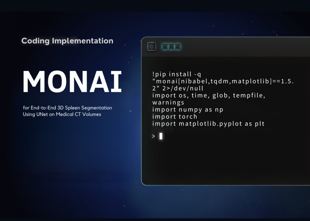
The foundation of any serious medical AI project lies in the correct installation of dependencies. We begin by securing MONAI alongside necessary libraries for numerical computation and visualisation. The code block below handles the installation of the specific version required for this workflow, ensuring compatibility across the ecosystem. We import essential modules from PyTorch, NumPy, and Matplotlib, alongside the core MONAI components required for dataset handling, data augmentation, network definition, and metric calculation. To maintain a clean execution environment, we suppress standard warnings, allowing the focus to remain strictly on the segmentation logic.
!pip install -q "monai[nibabel,tqdm,matplotlib]==1.5.2" 2>/dev/null
import os, time, glob, tempfile, warnings
import numpy as np
import torch
import matplotlib.pyplot as plt
from torch.amp import autocast, GradScaler
from monai.apps import DecathlonDataset
from monai.data import DataLoader, decollate_batch
from monai.networks.nets import UNet
from monai.networks.layers import Norm
from monai.losses import DiceCELoss
from monai.metrics import DiceMetric
from monai.inferers import sliding_window_inference
from monai.utils import set_determinism
from monai.transforms import (
   Compose, LoadImaged, EnsureChannelFirstd, EnsureTyped, Orientationd,
   Spacingd, ScaleIntensityRanged, CropForegroundd, RandCropByPosNegLabeld,
   RandFlipd, RandRotate90d, RandShiftIntensityd, AsDiscrete,
)
warnings.filterwarnings("ignore")
Defining configuration and data augmentation
Before loading data, we must establish the parameters that govern the training session. This includes selecting the computational device, defining the dataset root, and setting hyperparameters such as patch size, batch dimensions, and epoch counts. We also configure caching strategies to manage memory efficiently during the training phase. The code snippet below sets these variables, ensuring reproducibility by fixing the random seed. We then construct the preprocessing pipeline, which standardises CT volumes through orientation alignment and resampling. Crucially, we apply aggressive data augmentation during training-random flips, rotations, and intensity shifts-to prevent overfitting and improve the model’s generalisation capabilities, while keeping the validation pipeline static.
QUICK_RUN   = True
device      = torch.device("cuda" if torch.cuda.is_available() else "cpu")
root_dir    = tempfile.mkdtemp()
roi_size    = (96, 96, 96)
num_samples = 4
batch_size  = 2
max_epochs  = 15 if QUICK_RUN else 200
val_every   = 3
train_cache = 8 if QUICK_RUN else 24
val_cache   = 2 if QUICK_RUN else 6
set_determinism(seed=0)
print(f"Device: {device} | epochs: {max_epochs} | data dir: {root_dir}")
train_transforms = Compose(common + [
       image_key="image", image_threshold=0),
   RandFlipd(keys=["image", "label"], prob=0.2, spatial_axis=0),
   RandFlipd(keys=["image", "label"], prob=0.2, spatial_axis=1),
   RandFlipd(keys=["image", "label"], prob=0.2, spatial_axis=2),
   RandRotate90d(keys=["image", "label"], prob=0.2, max_k=3),
   RandShiftIntensityd(keys=["image"], offsets=0.10, prob=0.5),
   EnsureTyped(keys=["image", "label"]),
])
val_transforms = Compose(common + [EnsureTyped(keys=["image", "label"])])
Initialising datasets and training components
We now load the official Medical Segmentation Decathlon Task09 Spleen dataset. Using MONAI‘s DecathlonDataset class, we automatically download and manage the data split into training and validation sections. The training dataset receives the augmented transforms, whereas the validation set remains untouched to provide an unbiased assessment of performance. We wrap these datasets in PyTorch-style DataLoader objects to facilitate efficient batching and multi-threaded data loading. Following this, we configure the model architecture-a 3D UNet-along with the optimisation strategy. This includes the AdamW optimiser, a cosine annealing learning rate scheduler, and the DiceCE loss function, which is standard for medical segmentation tasks.
train_ds = DecathlonDataset(
   root_dir=root_dir, task="Task09_Spleen", section="training",
   transform=train_transforms, download=True, val_frac=0.2,
   cache_num=train_cache, num_workers=2, seed=0)
val_ds = DecathlonDataset(
   root_dir=root_dir, task="Task09_Spleen", section="validation",
   transform=val_transforms, download=False, val_frac=0.2,
   cache_num=val_cache, num_workers=2, seed=0)
train_loader = DataLoader(train_ds, batch_size=batch_size, shuffle=True,
                         num_workers=2, pin_memory=torch.cuda.is_available())
val_loader   = DataLoader(val_ds, batch_size=1, shuffle=False,
                         num_workers=1, pin_memory=torch.cuda.is_available())
print(f"Train volumes: {len(train_ds)} | Val volumes: {len(val_ds)}")
loss_fn   = DiceCELoss(to_onehot_y=True, softmax=True)
optimizer = torch.optim.AdamW(model.parameters(), lr=1e-4, weight_decay=1e-5)
scheduler = torch.optim.lr_scheduler.CosineAnnealingLR(optimizer, T_max=max_epochs)
scaler    = GradScaler("cuda", enabled=torch.cuda.is_available())
dice_metric = DiceMetric(include_background=False, reduction="mean")
post_pred   = Compose([AsDiscrete(argmax=True, to_onehot=2)])
post_label  = Compose([AsDiscrete(to_onehot=2)])
Executing the training loop
The core of the workflow is the training loop, which iterates through the defined epochs. During each epoch, the model processes cropped patches of the spleen dataset. We utilise automatic mixed precision (AMP) to accelerate computation and reduce memory consumption when a GPU is detected. The loop calculates the loss, performs backpropagation, and updates the model weights using the optimiser. At regular intervals, or at the conclusion of training, we switch the model to evaluation mode and perform inference using sliding-window techniques to ensure full coverage of the 3D volume. We track the Dice score throughout the process, saving the model checkpoint only when performance improves, ensuring we retain the best-performing weights.
best_dice, best_epoch = -1.0, -1
loss_hist, dice_hist, dice_epochs = [], [],Source Read original →Related articles