
Why your fine-tuning job takes longer than the FLOPs say
Our team analysed 272 production fine-tuning runs on NVIDIA H200 GPUs to find that standard FLOP calculations miss the mark by hours.
We have written a paper on the subject and will publish it on arXiv shortly. The study looks at how long jobs actually take on shared clusters compared to the theoretical time based on floating-point operations.
GPUs are expensive and scarce. Anyone running a shared cluster must decide daily which jobs run on which hardware and in what order. That plan depends entirely on accurate time estimates. If a job finishes early, the hardware sits idle. If it runs late, the queue behind it slips and experiments wait.
Accurate estimates allow for better planning rather than guesswork. Teams can decide what runs, when, and on how many GPUs with less wasted capacity. Most teams currently rely on a back-of-the-envelope FLOP calculation. The math says nine hours, but the job often finishes the next afternoon.
We wanted to know how far off that math is and if we could do better before a job starts. We took 272 real supervised fine-tuning jobs from our production pool of NVIDIA H200 GPUs. The total time consumed was about 7,382 GPU-hours. We compared analytical estimates against learned predictors.
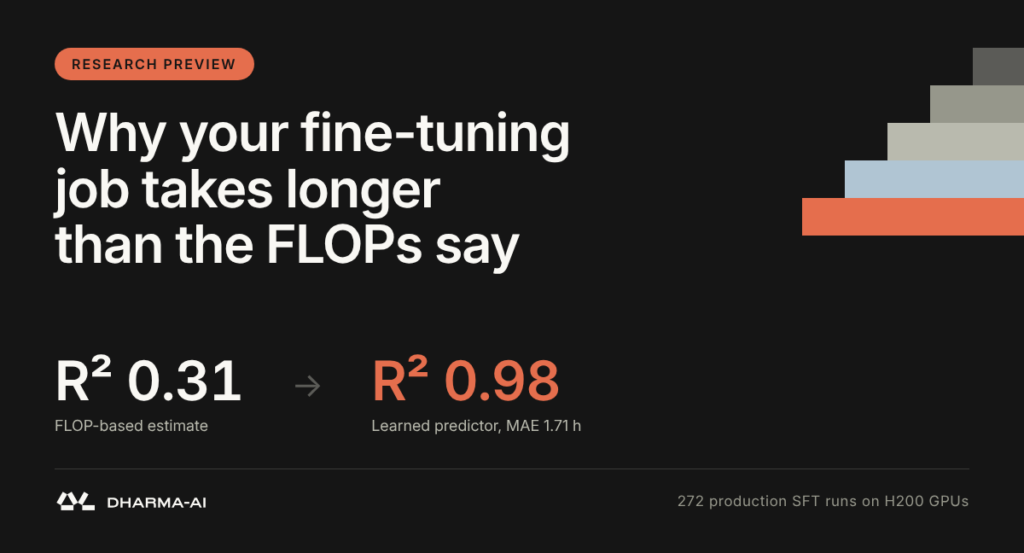
The short version is that the usual FLOP-based estimate explains little of what we observed. The R² score was 0.31 and the mean absolute error was 12.41 hours. A CatBoost regressor that only sees information available before dispatch reaches an R² of 0.98. It has a mean absolute error of 1.71 hours and a median error of 0.51 hours in 5-fold cross-validation. The gap comes from two things a closed-form estimate cannot do. The regressor sees more training-specific signals, such as evaluation cadence, checkpoint policy, per-GPU load and fine-tuning regime. It learns the nonlinear interactions between them from past runs.
The estimate everyone uses is compute-only
For a dense Transformer, training costs roughly 6 times P times D floating-point operations. P is the parameter count and D is the number of training tokens. Divide that by what your GPUs can deliver and you get a training-loop time:
T_theoretical = (6 · P · D) / (N_GPU · FLOPS_peak · MFU)
Here N_GPU is the number of GPUs, FLOPS_peak is the peak throughput of one GPU from its spec sheet, and MFU is the fraction of that peak the training actually achieves. Real jobs never run at peak because of memory traffic, communication and kernel inefficiencies. MFU typically sits somewhere between 30% and 60%. The right value for a given job is not known in advance.
This describes the optimisation loop. A job is more than its loop, though. Before the first step there is environment setup, model download and loading, and tokenisation. During training there are periodic evaluations and checkpoint uploads. At the end, the final model goes to object storage. On a multi-tenant cluster, all of it competes with other jobs for network and storage I/O.
These overheads depend on configuration and do not scale neatly with workload or GPU count. Two jobs with the same nominal compute can finish hours apart.
To keep the comparison fair, the FLOP baseline we test counts the scheduled evaluation tokens as well as the training tokens. We also sweep MFU over a wide range.
What we built
We treat end-to-end duration as a supervised regression problem. Given a feature vector built from the job configuration and model metadata, we predict the wall-clock time between the moment the job gets its GPUs and the moment it is done. Queue time is excluded.
Two design choices shaped the work:
- Everything is known before dispatch. Every input comes from the submitted configuration: hyperparameters, dataset sizes, model identifiers, GPU allocation. No runtime logs, no partial progress. That makes the prediction usable for scheduling.
- Features that expose the overheads. On top of the raw configuration we derive quantities such as num_eval_data, the total number of samples processed across all evaluation cycles. We also track num_saves and num_params_saved for checkpoint I/O, and per-GPU token volumes. The FLOP estimate itself, with MFU fixed at 0.45, goes in as one more feature called baseline_time. The model starts from the compute-only number and learns the corrections.
We compared Linear Regression, Ridge, XGBoost and CatBoost. Feature selection combined correlation filtering, mutual information and permutation importance across 18 candidate feature sets. We followed this with a grid search using MAE as the criterion. The final CatBoost model uses 24 features.
The data
- 272 SFT runs from the operational logs of a corporate production environment. These covered several model families up to 15 billion parameters, both LoRA and full fine-tuning, and a wide range of dataset sizes and hyperparameters.
- Shared infrastructure. Jobs ran on 1, 2 or 4 GPUs drawn from a pool of 8 to 32 H200s across 1 to 4 nodes. They ran alongside other training and inference workloads. The measured times include real contention.
- Durations ranged from 1.6 to 172.4 hours. The mean was 23.43 hours and the median was 15.29 hours.
- Stack: Hugging Face Transformers and Unsloth. We model the stack as a categorical feature and make no assumption about a fixed speedup between the two.
Distribution of end-to-end duration across the 272 runs shows a mean of 23.43 hours and a median of 15.29 hours.
Results
All numbers come from stratified 5-fold cross-validation. The first four rows are analytical and involve no fitting.
| Model | R² | RMSE (h) | MAE (h) |
|---|---|---|---|
| FLOP baseline (MFU 30%) | 0.31 | 20.45 | 12.41 |
| FLOP baseline (MFU 45%) | 0.18 | 22.38 | 13.01 |
| FLOP baseline (MFU 60%) | 0.01 | 24.56 | 14.62 |
| Calculon | −0.51 | 30.40 | 20.36 |
| Linear Regression | 0.69 ± 0.14 | 13.52 ± 4.23 | 7.52 ± 0.49 |
| Ridge | 0.73 ± 0.09 | 12.72 ± 3.70 | 7.23 ± 0.68 |
| XGBoost | 0.97 ± 0.01 | 4.18 ± 1.17 | 1.95 ± 0.32 |
| CatBoost | 0.98 ± 0.01 | 3.52 ± 0.78 | 1.71 ± 0.33 |
A few things stand out.
No single MFU value fixes the FLOP baseline. We swept MFU from 0.25 to 0.65. The best setting, 30%, still leaves a mean error above 12 hours on jobs that last 23 hours on average.
A more detailed analytical model does not close the gap. As a second baseline we took Calculon, an analytical performance model for LLM training from prior work. It builds an explicit layer graph and accounts for compute, memory traffic and inter-device communication. We extended the public implementation to cover LoRA, grouped-query attention, fused attention, bfloat16 and SwiGLU. Its estimates still correspond to a median of only 11% of the observed wall-clock time. That says nothing against Calculon as a step-level tool, which is what it was designed for. It shows how much of a production job happens outside the optimisation step.
Linear models help, and then stall. Ridge brings MAE down to 7.23 hours. The relationship between configuration and duration is not well captured by a purely linear model.
Gradient boosting does the heavy lifting. CatBoost and XGBoost land within one standard deviation of each other on every metric. We carry CatBoost forward because it has the lowest mean error across the board.
What the predictor relies on
CatBoost’s feature importance concentrates in a handful of features. Model and workload variables are there, as expected, but so are evaluation and checkpoint variables. num_eval_data, the total number of samples processed in evaluation over the life of the job, ranks first. It is followed by num_trainable_params, batch_eval_size_percent, num_all_params and num_gpus*batch_train_percent. num_params_saved is close behind. SHAP values tell the same story: high evaluation volume consistently pushes the predicted time up, while trainable parameter count has a nonlinear effect that only becomes large for the biggest models.
Mean feature importance of the CatBoost model across folds shows PredictionValuesChange.
Feature importance is not a causal claim. Still, the pattern lines up with how a job is actually spent. How often you evaluate, how large the evaluation set is and how many checkpoints you persist all shape the wall-clock time, alongside model and dataset scale. These are choices people often make by habit when writing a training config.
One caveat on reading the plots is that larger GPU allocations show positive contributions to predicted time. In our data, bigger allocations go with bigger jobs, so num_gpus acts partly as a proxy for job scale. It does not mean adding GPUs makes a job slower.
How wrong is it, and where
Looking at all 272 out-of-fold predictions, the median absolute error is 0.51 hours. 80% of predictions are within 2.20 hours and 90% are within 4.31 hours.