Allen AI releases custom embedding exports from OlmoEarth Studio

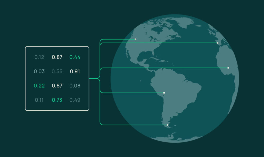
Users of Allen AI’s OlmoEarth Studio can now compute and export embedding vectors for Earth observation data. These numerical representations come from the organisation’s open source foundation models, with the source code and model weights available publicly alongside the research paper.

The export format is a Cloud-Optimized GeoTIFF (COG). These files are lightweight and designed for easy sharing. The system calculates vectors on demand rather than pulling them from a pre-computed global archive, ensuring the results reflect the specific conditions of your chosen area and time range.

Studio allows you to select the area of interest, time span, encoder variant, resolution, and imagery sources via the interface or API. If your application requires higher performance, the platform also supports supervised fine-tuning (SFT).

How to compute embeddings in Studio

The workflow mirrors any other prediction task. Configure a model, run it, and download the results. Several parameters tailor the output:

• Area of interest: Draw or upload any polygon; Studio handles imagery acquisition and tiling.
• Time span: 1-12 monthly periods.
• Encoder variant: Nano (128-dim, 1.4M params), Tiny (192-dim, 6.2M params), or Base (768-dim, 89M params).
• Spatial resolution: 10 meter, 20 meter, 40 meter, or 80 meter per pixel.
• Imagery sources: Sentinel-2 L2A, Sentinel-1 RTC, or both.

Studio delivers a COG with one band per embedding dimension. Vectors are stored as signed 8-bit integers (int8). Values range from -127 to +127, with -128 reserved for nodata. To recover floating-point vectors, see dequantize_embeddings in olmoearth_pretrain.

Because everything is computed on demand, your embeddings reflect exactly the conditions you care about. You can generate monthly embeddings to capture seasonal dynamics, not just annual snapshots.

Use cases

The examples below all use OlmoEarth-v1-Tiny (192-dim) embeddings at 40-meter resolution with Sentinel-2 L2A composites. Tiny is a lightweight encoder but still highly performant; for your own applications, you can swap it for a larger variant at the cost of higher compute and storage.

Similarity search

Pick a query pixel, extract its embedding, and compute cosine similarity against every other pixel. The result is a heatmap showing where the landscape looks most and least like your query pixel.

This query sits near the Merced urban center in California. Urban fabric and road corridors light up coherently while agricultural parcels stay dark. The model distinguishes built-up surfaces from cropland without any labels.

Switching the query to a small agricultural window, we define the query vector as the mean of the embedding vectors over that window, then pull Sentinel-2 imagery at the highest- and lowest-similarity locations to see what the model treats as similar and dissimilar.

The most similar patches (0.89 and above) are all agricultural parcels with irrigated fields. The least similar (around zero) are an airport with surrounding bare ground, a reservoir with dry terrain, and arid rangeland. No training data, no labels, just a dot product in embedding space.

Few-shot segmentation

Similarity search tells you “where is it like this?” but sometimes you need discrete labels across a region. Because the representations are already rich, a simple linear classifier can produce a wall-to-wall land-cover map from very few labeled pixels.

To test this, we labeled just 60 pixels (20 per class) over Ca Mau, Vietnam, a coastal mangrove region. Using ESA WorldCover 2021 as the label source for three classes (mangrove, water, other), we randomly sampled 20 pixels per class, trained a logistic regression with per-feature standardization, and predicted every pixel in the region.

From 60 labeled pixels, the classifier produces a coherent map with weighted F1 = 0.84. Mangrove stands, tidal channels, and open water are delineated across the entire region. The classifier saturates quickly: increasing from 30 to 300 labels barely changes accuracy, because the embeddings are doing most of the heavy lifting.

This is a linear probe, a standard evaluation for foundation models. The fact that a logistic regression over 192 dimensions recovers land-cover boundaries from so few labels means the Tiny encoder has organized these ecological distinctions during pretraining. Larger variants (Base, 768-dim) encode even richer representations.

If you have ground-truth polygons, field survey points, or a coarse existing map, you can train a similar classifier and produce a wall-to-wall map for your own region of interest.

Change detection

Because Studio can generate embeddings at any temporal resolution (monthly through annual), you can compare two time periods directly to identify where surface conditions have changed. Below, we computed monthly Sentinel-2 embeddings for the same region in September 2023 and September 2024 and measured per-pixel cosine distance. The Park Fire (July-September 2024) burn scar in Butte County, California lights up immediately.

No labels or training required—just two embedding COGs and a few lines of Python.

Unsupervised exploration

Sometimes you have no query location or reference labels. You just want to understand what structure exists in the embeddings. Principal Component Analysis (PCA) is a clean way to do this: reduce to three dimensions, map to R/G/B, and display as a false-color image. Similar embeddings get similar colors automatically.

Flevoland, in the Netherlands, is a reclaimed polder landscape with a regular grid of agricultural parcels. The PCA false-color image reproduces those boundaries with high fidelity. Different crop types, water bodies, and urban areas each get distinct hues. The embedding has internalized landscape structure without ever being told what a parcel or crop is.

This kind of unsupervised view is a quick way to see what structure the model has picked up across your area of interest.

From export to insight

Similarity search, few-shot segmentation, change detection, and PCA exploration are simple operations on standard raster data that run in seconds. The power comes from the embeddings: learned representations that compress earth observation data into vectors capturing rich information about each location from many sensors and millions of training examples.

Custom embedding exports are available now. Create a project, configure an embeddings model, and compute your embeddings. The exported GeoTIFF works with any geospatial tool: QGIS, GDAL, rasterio, or your own scripts. For end-to-end code reproducing the examples in this post, see the embeddings tutorial, which includes working code for similarity search, few-shot segmentation, change detection, and PCA visualization. To get hands-on without any local setup, try the Colab notebook.

Fine-tuning

The examples in this post all use frozen embeddings with no task-specific training. Embeddings are a great entry point for generating results, they work well in resource-constrained environments, and are easy to share. For applications that require higher performance, OlmoEarth Studio also supports SFT, training a task-specific model head on your own labels, which typically outperforms linear probes on frozen features.

Limitations

While we are always working to improve our pretraining approaches, it’s important to check the quality of the embeddings for your use case using some of the techniques described above. Performance also depends on the quality of the input imagery—persistent cloud cover, atmospheric artifacts, or missing observations in the composite period can affect the resulting vectors.

Sentinel-2 L2A imagery from the European Space Agency, accessed via Microsoft Planetary Computer. ESA WorldCover 2021 v200 for mangrove reference. The global clustering visualization uses OlmoEarth-v1-Base (768-dim) with seasonal Sentinel-2 composites at patch size 8, instance-level embeddings over 1.1M pretraining samples.